
In today's chapter we will talk about gradient descent, an optimization algorithm that plays a key role in the field of Machine Learning. As we mentioned in previous chapters, "Neural Networks and Deep Learning. Chapter 2: The Neuron" and "Neural Networks and Deep Learning. Chapter 1: Prelude", a neuron can be seen as a mathematical function that receives some input values and gives an output value. In addition, we also saw that these values are affected by some parameters or weights. These parameters determine the influence that an input value has on the function. In this way, these weights have a direct importance in the error that our neural network can have in its predictions. It is here where the cost function comes into play, which is the one that tries to quantify the error between the prediction and the real value, in order to optimize the parameters of the neural network. By means of gradient descent we will try to minimize this cost function as we will explain below.
Optimization: Gradient of a function
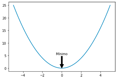
As we have seen in the previous section our mission in the following will be to find the minimum value of the cost function. Finding the minimum of a function is a very common task in mathematical analysis. Normally, the common way to attack the problem of finding the minimum point is reduced to find the point (or points) where the derivative of the function is equal to zero. In fact, it is relatively easy when we encounter convex functions like the following:
However, in most cases we will encounter high-dimensional and more complex functions. In these cases finding the minimum can be a rather tedious task since it involves solving a presumably large number of partial derivatives. This happens, for example, in the following case:
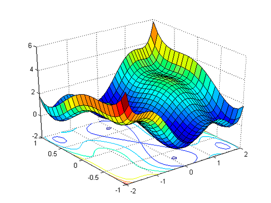
However, all is not lost. This is where the gradient of the function comes into play.
Definition: We call gradient or gradient vector of a function the vector generalization of the derivative. It is a vector of the same dimension as the function.
"It is also convenient to remember that the derivative contains information about the slope of our function. Specifically, it tells us the direction of maximum growth of the function. We present then the formula for the gradient of a function f with n parameters x1, ..., xn"
Logic of gradient descent
Now that we know that the gradient of a function contains information about the slope of that function at a point, it is time to illustrate the logic of the algorithm using a classic example.
Suppose we are at a random point in a mountain range with several mountains of different heights where visibility is zero. We are lost and want to return to the lowest point of the valley, but the fog makes it impossible to see. Perhaps in such a situation the most intelligent solution is the following:
- Detect the direction in which you are descending the most. We could take a step in each of the four directions to finally choose the one in which we are descending the most. In practice this is analogous to calculating the gradient, since by means of this we can detect the direction of maximum growth and, consequently, the direction of maximum decrease.
- Once we have detected the direction of decrease we walk one or more steps in that direction.
In this way we repeat both operations until we reach the minimum point. But, there is an important question... How big should be the steps we take in each iteration? This is where the concept of Learning Rate appears.
Learning Rate
As we have already mentioned, we can understand the Learning Rate as that parameter that indicates how long the steps we take while descending have to be. In technical terms, this means how much the gradient affects the update of our parameters.
A priori, it seems reasonable to follow the following strategy:
- If the gradient indicates that the slope is steep then we will take a very long step to take advantage and descend as much as possible.
- If the gradient indicates that the slope is not very steep, we will take a shorter step.
In conclusion, we will step proportionally to the gradient, but to control this proportion we will use the learning rate.
In the following images we can see what happens in the gradient descent algorithm for the same cost function but different learning rate values:
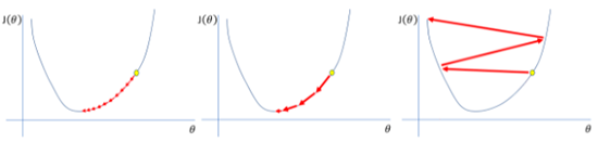
- A very small learning rate, like the one in the figure on the left, can make us converge to the minimum, but it entails a high number of steps. This in practice translates into a high computational cost since it means that we will have to perform a large number of derivatives. Also, a small learning rate can make us converge to local minima instead of absolute minima.
- A learning rate that is too high, like the one in the figure on the right, can make us diverge. The steps are so long that it becomes very difficult to enter the minimum cost zone.
Perhaps we can see it more clearly in the following animation, which also illustrates the difference between the different techniques currently used to dynamically adjust the learning rate.

At this point we are ready to learn how to endow a neural network with that intelligence or ability to readjust its parameters. But, that will be in the next chapter!