

As we saw in the previous chapter, Neural Networks and Deep Learning. Chapter 3: Gradient descent, allowed us to optimise the cost function according to the neuron parameters. In this way we are able to find a combination of these parameters that minimises the error in the predictions of our network. At this point, our main objective is that the network becomes autonomous when learning and that we do not have to readjust these parameters. This is where the Backpropagation algorithm comes into play, an algorithm described in 1986 in "Learning representations by back-propagating errors", an article that would bring neural networks back to life.
Motivation of the Backpropagation algorithm
If we go back to the first two chapters, we recall that neurons combine with each other to form a complex structure that we call a neural network.
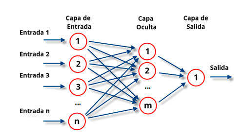
In this way, and according to the image notation, an input parameter of any of the n neurons of the first layer can affect the output of any of the neurons of the m-th hidden layer, and consequently the final result. Moreover, recall that the computation of the gradient became complicated when the number of parameters is high due to the computation of so many partial derivatives.
Here's the kit de la question. In a neural network, the error of the upstream layers depends directly on the error of the downstream layers, which is why we can analyse and optimise thepropagation of the errorbackwards in the network. In this way we can also assume that if we have the error controlled for a neuron N of the m-th layer, then the parameter settings for each of the neurons of the m-1 previous layers that have influence on the input parameters of our neuron N,also have little influence on our final error. We will see this more clearly with an example below.
Example of Backpropagation
Let's suppose that a company has had bad results in the first quarter of the year. We will be interested to know what has caused these results. As is normal, there are different departments with different employees in each of them. All these employees have more or less family, social or health problems, which inevitably have an impact on their good or bad performance. This in turn ends up having more or less relevance on the company's results, as we can see in the diagram below.
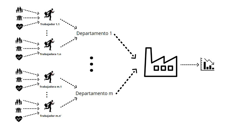
The logic behind the Backpropagation algorithm tells us that if, for example, a department has not had much influence on this negative quarterly result then we can assume that the workers in this department, and their daily life problems, have not been relevant in this respect either. This means that when computing the gradient decline we can save all partial derivatives involving the branch of this department. On the other hand, if we detect the department that has had an influence on the bad results, it would be worthwhile to go deeper to get to the root of the problem. In this case we might discover a 'problem' at any of the stages, perhaps the whole department has failed to work as a team, or perhaps a key worker had a bad day because of an argument with friends.
Mathematics of the Backpropagation algorithm
A priori, the mathematics involved in this algorithm may seem very cumbersome due to the notation and the computational cost involved. Nothing could be further from the truth, we just need to be clear about the following concepts:
Composition of functions:
In a simple way, we will say that given two real functions f and g. We call the new function defined by g, or f(x) = g(f(x)), a composite function of f and g.
Example:
If f(x) = 5x and g(x)=x2, then g or f(x) = g(f(x)) = (5x)2 = 25x2.
Chain rule:
This is a very common formula in calculus to obtain the derivative of composite functions such as the one we have just seen. Mathematically this rule says that (g or f)'=(g' or f) f'.
Example:
Following the previous example: f'(x) = 5 y, calling f(x) = y, g(f(x))'=g(y)'=2y, since y = 5x, g(f(x))'=2(5x). Then, according to the chain rule, the result is (g or f)'(x) = 50x.
We could go into notation, but we just have to assume that each path in the neural network is a composition of functions. Then, by applying the above two concepts we can measure the influence of any parameter of our network on the prediction error (the partial derivative of the cost function with respect to the parameter).
So much for the technical part and the mathematics of neural networks. In what follows we will look at concepts such as convolutional neural networks and their applications - don't miss it!